7.11 DESIGN OF SERVOVALVES
Fixed-area-type regulating devices have definite limitations. For instance, an orifice regulates flow and pressure only under specific conditions of flow, but does not function under other conditions. By contrast, variable-areatype devices will function under both dynamic and static conditions. Classified according to their function, the most frequently used variable-area-type pressure and flow regulating devices for rocket engines can be grouped into- (1) Throttle valves (including valves for thrust and control) (2) Gas pressure regulators (3) Liquid flow regulators
Throttle valves have been discussed in section 7.8. Detail on gas pressure and liquid flow regulators will be found in sections 7.12 and 7.13. Many of these devices use some form of fluid-pressure-operated actuator. The position of the actuator, and thus the area of the controlling valve opening, is effected by applying a pressure differential across the actuator piston or diaphragm, by means of various types of servo pilot valves, which will be discussed. The function of a servovalve is similar to that of an on-off pilot valve, except that it can continuously vary the pressure or flow rate of the actuating fluid to control the desired actuator position. In a pneumatic actuating system, the servovalve operates as a pressure control device. It functions as a flow control device in hydraulic systems. In rocket engine applications, where usually only low-power electrical signals or sensing pressure forces are available to operate the valves, servovalves with very high gain characteristic are required. Three basic servovalve types are most frequently used: the flapper-nozzle type (fig. 7-55), the spool type (fig. 7-56), and the poppet type (fig. 7-57). They are used independently, or jointly, to form a twostage servovalve in which the flapper-nozzle valve acts as a pilot valve for the spool valve. A typical example was presented in figure 7-9.
General Design Considerations for Servovalves:
(1) Type of control fluid (gas or liquid) and its conditions (pressure and temperature) (2) Systems gain: In some applications the ratio between electrical quiescent input power to the valve coils and the maximum valve output (as defined by eq. (7-17)) is as high as (3) Bandwidth and frequency response; dynamic stability (4) Minimum bleed of control fluic (5) Simplicity of construction and line connections (6) Compatibility with environmental conditions: temperature, humidity, acceleration, and vibration. The open-loop gain and phase shift versus frequency characteristics of a typical servovalve and driving amplifier combination are shown in figure 7-54. These characteristics are obtained by applying an input signal to the servoamplifier from an oscillator. The amplifier drives the valve by means of a current input to the valve transducer coil (torque motor). In turn, the valve controls the flow of working fluid to the actuator which produces the desired load force. The voltage output from a potentiometer attached to the actuator is then compared to the amplifier input. Instead of electrical feedback, mechanical feedback may be employed. (See sec. 7.5, "Engine Thrust Vector Control.")
Flapper-Nozzle-Type Servovalves
The flapper-nozzle-type servovalve is essentially a variable orifice or nozzle. Figure illustrates schematically the operation of a typical double-bleed unit. Actuating fluid is supplied at a constant pressure or flow rate. When an input signal is fed to the torque motor from a servoamplifier, the electric signal is converted into a mechanical force. The resultant deflection of the flapper is proportional to the input signal and causes the flow of actuating fluid to increase at one nozzle, and to decrease at the
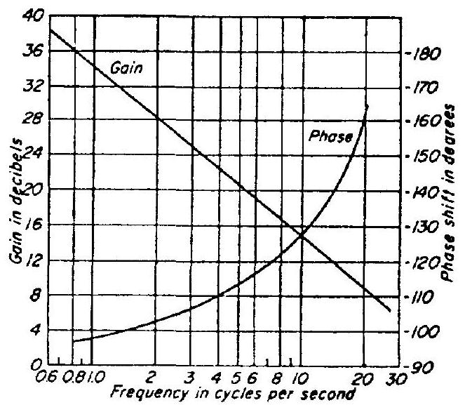 Figure 7-54.-System characteristics of a typical servovalve and driving amplifier combination.
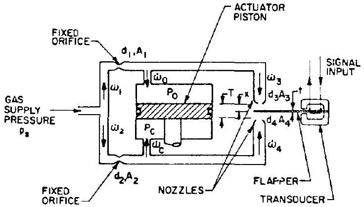 Figure 7-55.-Schematic of a typical flapper-nozzle-type pneumatic servovalve.
other. An increased flow reduces the fluid pressure (compressible fluid) or fluid volume (incompressible fluid) on the corresponding side of the actuator piston. Correspondingly, the fluid pressure or fluid volume on the other side of the piston increases. The resultant pressure differential across the actuator piston causes it to move in the desired direction. The flappernozzle valve is also applicable to servo systems with single-control nozzle bleed. Here, the actuator position is controlled by regulating the actuating fluid on one side of the piston or diaphragm only. This is analogous to the singlebleed pneumatic poppet servovalve (fig. 7-57).
Flapper-nozzle valves are particularly suitable as pilot valves for larger servovalves (see fig. 7-9). Because the transducers or torque motors for these valves require rather low power levels, they usually consist of coil relays exerting forces of only a few ounces. The effect of the flapper spring rate is often counterbalanced by the gradient of the magnetic force developed in a properly designed transducer or by mechanical means. To prevent spreading of the jets leaving the nozzles and to ease the rate balancing between flapper spring and transducer magnetic forces, the travel of the flapper should be kept reasonable small.
Equations (7-22) and (7-24), which describe the flow of liquids and gases through orifices and nozzles, are applicable to the design calculations of flapper-nozzle valves. Two conditions may exist for the flow through the nozzles of a flapper-nozzle valve: first, when the restriction is determined by the position of the flapper; and secondly, when the flapper has moved far enough from the nozzle for the flow to be restricted by the throat area of the nozzle. Most designs are based on the first condition. The effective (ring shaped) flow area then is
where
Sample Calculation (7-9)
The following dimensions and data are defined for a flapper-nozzle pneumatic servovalve (schematically shown in fig. 7-55), which is used as a pilot valve of the servo control valve attached to the main oxidizer valve of the stage engine:
Helium supply pressure, , and temperature corresponding diameters and flow areas of fixed orifices and nozzles flow rates through fixed orifices and nozzles, and to and from the actuator, lb/sec compressibility factors of the flows through the orifices and nozzles Flow coefficient of the orifices and nozzles,
Distance between the two nozzles,
=thickness of the flapper At the neutral or equilibrium position of the servovalve:
The pressures in the actuators, psia The bleed through nozzles, lb/sec Determine: (a) The dimensions of fixed orifices and nozzles, and of distance . (b) The pressure differential across the actuator piston when the flapper is deflected downward 0.001431 inch from its neutral position, and the flow rates and to and from the actuator are (as governed by the speed of the piston).
Solution
(a) Since the gas flow through the nozzles is discharged to ambient, it is assumed that the pressure ratio across the nozzles will always be less than critical (sonic flow).
From figure 7-53, . From equation (7-24), the following correlations are established:
The flow areas of fixed orifices and flapper nozzles (eq. (7-27)) are:
When the valve is at neutral position, the actuator is at rest, and
Since under these conditions, the pressure ratio across the fixed orifices is .
From figure 7-53,
Since
(b) When the flapper is deflected downward 0.001431 inch from its neutral position, the displacement of the flapper from the upper nozzle
With the flapper deflected
The flow rate through the upper nozzle, , is now equal to the fixed orifice flow rate , plus the flow rate from the actuator ; thus
We use a trial-and-error method to find these values for and , which will satisfy the above correlations and figure 7-53. We find that
Checking the results for a pressure ratio of
a value of 2.687 is derived from figure 7-53; thus
With the flapper deflected
The flow rate through the lower nozzle, , is equal to the fixed orifice flow rate , minus the flow rate to the actuator, :
We use again a trial-and-error method to obtain the values for and which will satisfy the above correlations and figure 7-53. We have found that
Thus the pressure differential across the actuator piston
Spool-Type Servovalves
The spool-type servovalve (schematically shown in fig. 7-56) is basically a four-way valve. A cylindrical valve spool is accurately fitted into valve inserts, which in turn are shrunk into the valve body. Both inserts and spool are made of hardened alloy steels. The thickness of the inserts in the axial direction, and thus the location of the ports, is held to very close tolerances by lapping their faces. The outside diameter of the inserts is accurately ground for a tight seal with the valve body. The surfaces of their axial passages are also lapped. The diametral clearance between insert and spool is of the order of 0.0002 inch, at which the spool must still slide freely. The axial location of the spool lands must also be closely controlled. To minimize leak flow in the neutral position, the spool lands may be designed for slight overlap. As a rule, leak flows are less when the spool is displaced, due to better isolation of the drain lines. A typical leak flow rate in neutral position is 0.5 gpm.
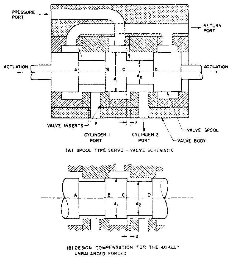 Figure 7-56.-Spool-type servovalve.
Although the spool valve theoretically is force balanced, hydrodynamic and friction forces cause relatively large loads which must be overcome. Refer to figure (a). Due to the difference in flow velocities, the static pressure at face will be less than that at face . Similarly, the pressure is less at face than at face . This results in two approximately equal axial forces, both of which tend to move the valve spool to the right so as to close the valve. These unbalanced axial forces can be compensated by design remedies. One is to increase diameter (as shown in fig. 7-56(b)). It is recommended that the maximum control port flow area (where spool displacement, in) be just less than twice the annular area between spool diameters and . As a result, the flow velocity along the spool is substantially increased and the axial forces on faces and are considerably reduced.
The difference between minimum flow rate (leak flow in neutral position) and maximum flow rate (actuator in motion) is substantial. Various means of adjustment may be employed, such as simple relief bypass valves, or the pump output may de adjusted. For instance, in a piston pump operated by a wobble plate, the pitch of the plate may be adjusted as a function of pressure to give strokes varying from maximum to zero.
The correlation between pressure drop and flow in a spool valve is not as predictable as one might expect from a sharp-edged orifice. Experimental data are required to verify a design. Equation (7-24) for gas flow orifices may be used to approximate the flow through a pneumatic spool valve, where orifice area and flow coefficient . For a spool valve using hydraulic oil or RP-1 as the actuating fluid, the following empirical equation applies:
where valve pressure drop, psi valve volumetric flow rate, in spool displacement, or valve opening, in density of the liquid,
Sample Calculation (7-10)
The following design data are given for a spool-type hydraulic servovalve (shown schematically in fig. 7-56):
RP-1 is supplied at pressure Valve pressure drop and flow characteristics may be obtained from equation (7-28), for the following design constants:
Maximum spool displacement, in Determine the flow rate , pressure drop , and output of the valve at maximum displacement.
Solution
Substitute , and into equation (7-28)
From equation (7-17), the valve output
To find the maximum valve output design point, this expression is differentiated and set equal to zero
or
It should be noted that stabilized flow conditions rarely exist, because of mass inertias limiting acceleration and deceleration, and feedback effects.
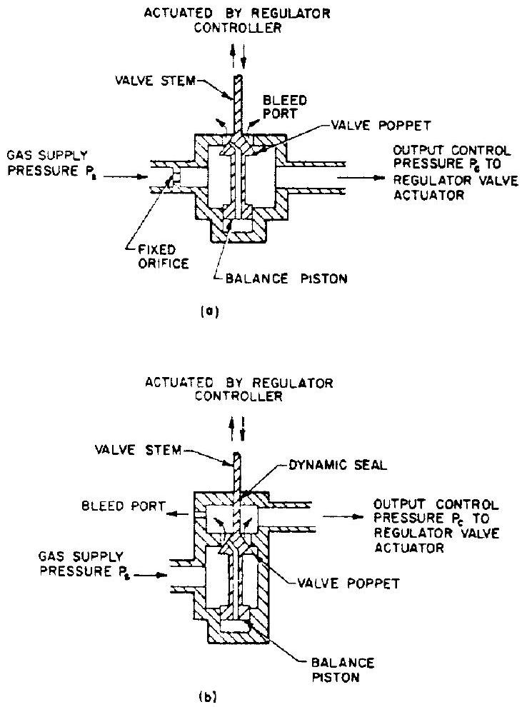 Figure 7-57.-Schematics of typical single-bleed, poppet-type, pneumatic servovalves used in gas pressure regulators.
Single-Bleed, Poppet-Type Servovalves
The single-bleed, poppet-type servovalve operates as a variable orifice like the flappernozzle valve. Figure presents, schematically, the principle of operation of typical single-bleed, poppet-type, pneumatic servovalves as used in gas pressure regulating services. Two basic configurations are in use. The first (fig. 7-57(a)) effects output control pressure regulation through variation of bleed port flow area. In the second (fig. 7-57(b)), the bleed port area is fixed. Here, is regulated by varying the supply gas flow rate.
The selection of configuration depends on application. To minimize unbalance forces, a balance piston is usually attached to the valve poppet. The area of the balance piston is made equal to the projected area of the poppet seat diameter, less that of the valve stem.